Classifying messy documents: A common-sense approach (Part II)

This post was kindly contributed by SAS Users - go there to comment and to read the full post.

In Part I of this blog post, I provided an overview of the approach my team and I took tackling the problem of classifying diverse, messy documents at scale. I shared the details of how we chose to preprocess the data and how we created features from documents of interest using LITI rules in SAS Visual Text Analytics (VTA) on SAS Viya.

In this second part of the post, I’ll discuss:

scoring VTA concepts and post-processing the output to prepare data for predictive modeling
building predictive models using SAS Visual Data Mining and Machine Learning
assessing the results

Scoring VTA Features

Recall from Part I, I used the image in Figure 1 to illustrate the type of documents our team was tasked to automatically classify.

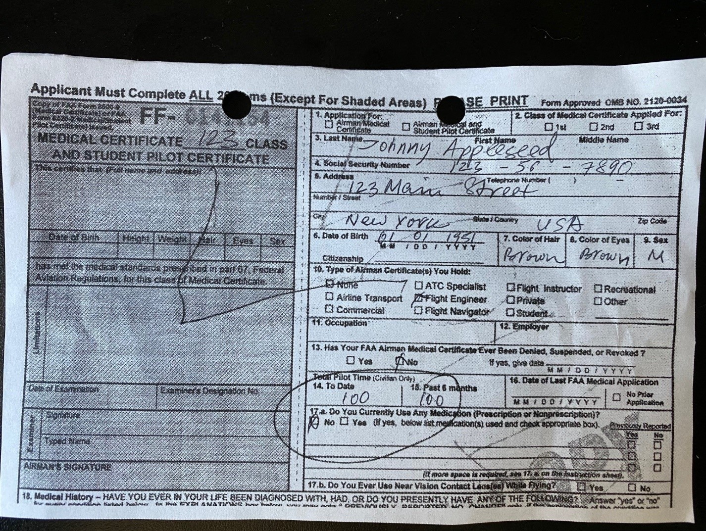
Figure 1. Sample document

I then demonstrated a method for extracting features from such documents, using the Language Interpretation Text Interpretation (LITI) rules. I used the “Color of Hair” feature as an example. Once the concepts for a decent number of features were developed, we were ready to apply them to the corpus of training documents to build an analytic table for use in building a document classification model.

The process of applying a VTA concept model to data is called scoring. To score your documents, you first need to download the model score code. This is a straightforward task: run the Concepts node to make sure the most up-to-date model is compiled, and then right-click on the node and select “Download score code.”

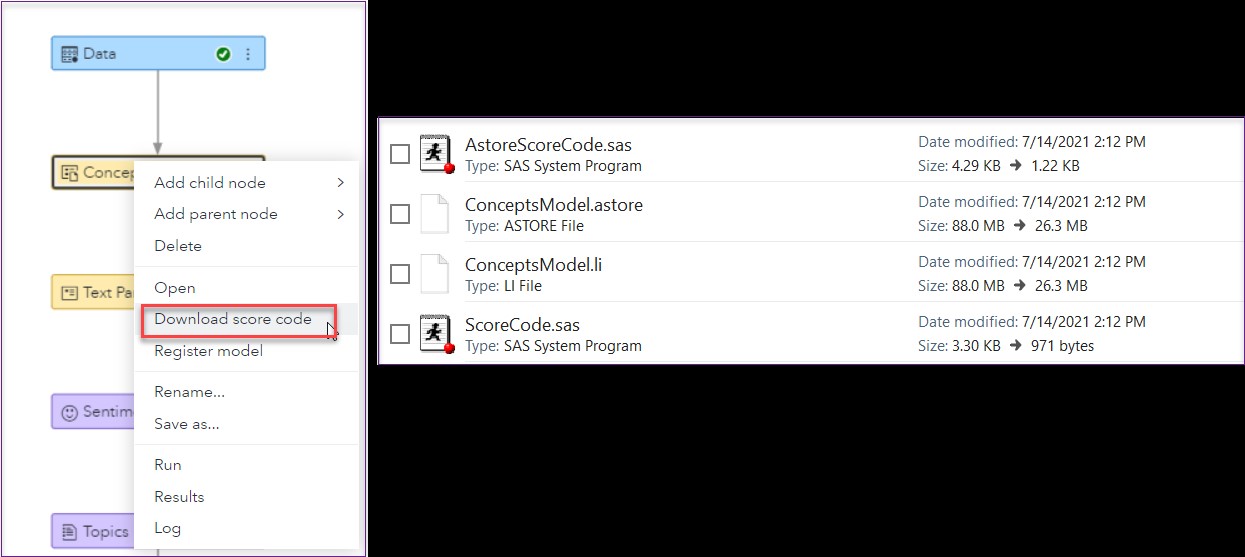
Figure 2. Exporting concept model score code

You will see four files inside the downloaded ZIP file. Why four files? There are two ways you can score your data: using the the with the concepts analytics store (astore) or the concepts model. The first two files you see in Figure 2 score the data using the astore method, and the third and fourth file correspond to scoring using the concept .li binary model file.

If you are scoring in the same environment where you built the model, you don’t need the .li file, as it is available in the system and is referenced inside the ScoreCode.sas program. This is the reason I prefer to use the second method to score my data – it allows me to skip the step of uploading the model file. For production purposes though, the model file will need be copied to the appropriate location so the score code can find it. For both development and production, you will need to modify the macro variables to match the location and structure of your input table, as well as the destination for your result files.

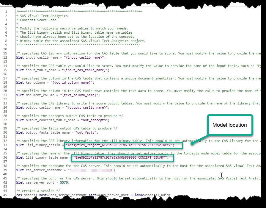
Figure 3. Partial VTA score code – map the macro variables in curly brackets, except those in green boxes

Once all the macro variables have been mapped, run the applyConcept CAS action inside PROC CAS to obtain the results.

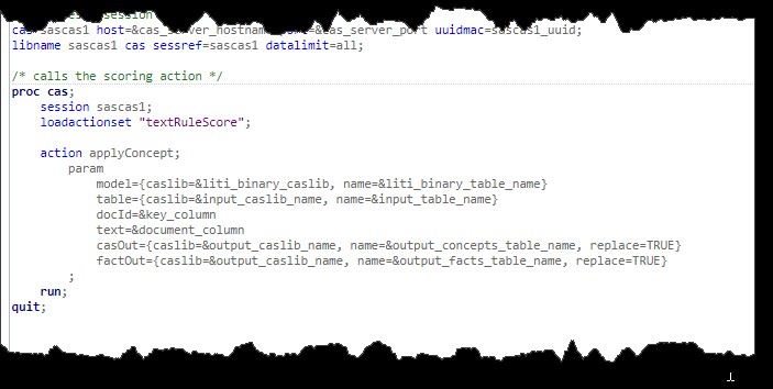
Figure 4. Partial VTA score code

Depending on the types of rules you used, the model scoring results will be populated in the OUT_CONCEPTS and/or OUT_FACTS tables. Facts are extracted with sequence and predicate rule types that are explained in detail in the book I mentioned in Part I. Since my example didn’t use these rule types, I am going to ignore the OUT_FACTS table. In fact, I could modify the score code to prevent it from outputting this table altogether.

Looking at the OUT_CONCEPTS table, you can see that scoring returns one row per match. If you have multiple concepts matching the same string or parts of the same string, you will see one row for each match. For troubleshooting purposes, I tend to output both the target and supporting concepts, but for production purposes, it is more efficient to set the behavior of supporting concepts to “Supporting” inside the VTA Concepts node, which will prevent them from showing up in the scored output (see Figure 5). The sample output in Table 1 shows matches for target concepts only.

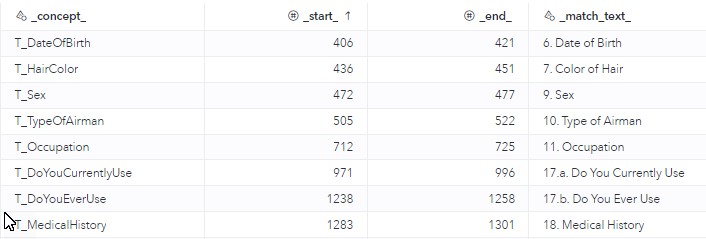
Table 1. OUT_CONCEPTS output example

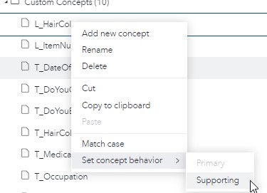
Figure 5. Setting concept behavior to supporting

Completing Feature Engineering

To complete feature creation for use in a classification model, we need to do two things:

Convert extracted concepts into binary flags that indicate if a feature is present on the page.
Create a feature that will sum up the number of total text-based features observed on the page.

To create binary flags, you need to do three things: deduplicate results by concept name within each record, transpose the table to convert rows into columns, and replace missing values with zeros. The last step is important because you should expect your pages to contain a varying number of features. In fact, you should expect non-target pages to have few, if any, features extracted. The code snippet below shows all three tasks accomplished with a PROC CAS step.

/*Deduplicate OUT_CONCEPTS. Add a dummy variable to use in transpose later*/
data CASUSER.OUT_CONCEPTS_DEDUP(keep=ID _concept_ dummy);
	set CASUSER.OUT_CONCEPTS;
	dummy=1;
	by ID _concept_;
	if first.concept_ then output;
	run;
 
/*Transpose data*/
proc transpose data=CASUSER.OUT_CONCEPTS_DEDUP out=CASUSER.OUT_CONCEPTS_TRANSPOSE;
	by ID;
	id _concept_;
	run;
 
/*Replace missing with zeros and sum features*/
data CASUSER.FOR_VDMML(drop=i _NAME_);
	set CASUSER.OUT_CONCEPTS_TRANSPOSE;
	array feature (*) _numeric_;
	do i=1 to dim(feature);
		if feature(i)=. then feature(i)=0;
	end;
	Num_Features=sum(of T_:);
	run;
 
/*Merge features with labels and partition indicator*/
data CASUSER.FOR_VDMML;
merge CASUSER.OUT_CONCEPTS_TRANSPOSE1 
	  CASUSER.LABELED_PARTITIONED_DATA(keep= ID target partition_ind);
by ID;
run;

To create an aggregate feature, we simply added up all features to get a tally of extracted features per page. The assumption is that if we defined the features well, a high total count of hits should be a good indicator that a page belongs to a particular class.

The very last task is to merge your document type label and the partitioning column with the feature dataset.

Figure 6 shows the layout of the table ready for training the model.

Figure 6. Training table layout

Training Classification Model

After all the work to prepare the data, training a classification model with SAS Visual Data Mining and Machine Learning (VDMML) was a breeze. VDMML comes prepackaged with numerous best practices pipeline templates designed to speed things up for the modeler. We used the advanced template for classification target (see Figure 7) and found that it performed the best even after multiple attempts to improve performance. VDMML is a wonderful tool which makes model training easy and straightforward. For details on how to get started, see this free e-book or check out the tutorials on the SAS Support site.

Figure 7. Example of a VDMML Model Studio pipeline

Model Assessment

Since we were dealing with rare targets, we chose the F-score as our assessment statistic. F-score is a harmonized mean of precision and recall and provides a more realistic model assessment score than, for example, a misclassification rate. You can specify F-score as your model selection criterion in the properties of a VDMML Model Studio project.

Depending on the document type, our team was able to achieve an F-score of 85%-95%, which was phenomenal, considering the quality of the data. At the end of the day, incorrectly classified documents were mostly those whose quality was dismal – pages too dark, too faint, or too dirty to be adequately processed with OCR.

Conclusion

So there you have it: a simple, but effective and transparent approach to classifying difficult unstructured data. We preprocessed data with Microsoft OCR technologies, built features using SAS VTA text analytics tools, and created a document classification model with SAS VDMML. Hope you enjoyed learning about our approach – please leave a comment to let me know your thoughts!